Using Knowledge Accounting for Project Success
Knowledge Gaps & the Law of Requisite Variety
Introduction
When starting a new project:
- Identify the skills needed for the project.
- Determine the expertise required to complete the work successfully.
- Assess the skills gap. Compare the required skills to the existing skills within the team.
- Evaluate the project skills readiness of the teams involved.
- Determine the budget required to acquire the necessary skills.
- Compare the required budget to the allocated budget and assess what is financially feasible.
- Prioritize training efforts based on the impact of specific skill gaps on project success.
- Ensure the project starts at an acceptable risk level, balancing skills readiness, budget, and timeline constraints.
Identifying the Skills Needed for a Project
Identifying the skills needed for a project is a critical first step in Knowledge Accounting.
There are several methods to systematically determine the required skills. Each method has its strengths and works best in different contexts. A combination of all of the approaches is presented in the Framework for Identifying Skills Needed for a Project in the Appendix to ensure a comprehensive skill identification process.
After following the framework, we should have a comprehensive list of required skills presented in a matrix D.
-
Rows in D → Different skill profiles required for the project.
- Each row represents a Skill Profile (distinct task, role, or requirement needed for the project).
- Example: A project might need Backend, Frontend, and DevOps expertise, and each row represents a required combination of these skills.
-
Columns in D → Different types of skills.
- Let's say the 3 columns represent:
- Backend Development
- Frontend Development
- DevOps
- Thus, each row is a combination of skill levels required for a specific role/task.
Example Matrix 𝐷 - Required skills for project X.
|
Role |
Backend |
Frontend |
DevOps |
|
Role 1 |
1 |
0 |
2 |
|
Role 2 |
0 |
1 |
1 |
|
Role 3 |
1 |
1 |
0 |
Example interpretation:
- Skill Profile 1: Requires 1 unit of Backend, 0 of Frontend, and 2 of DevOps.
- Skill Profile 2: Requires 0 Backend, 1 Frontend, and 1 DevOps.
- Skill Profile 3: Requires 1 Backend, 1 Frontend, and 0 DevOps.
Individual Skill Profiles
Next we prepare a matrix R of individual skill profiles for teams i.e. existing skills within the teams. We present those in another matrix R
- Rows in R → Individual team members.
- Each row corresponds to the skills possessed by a team member.
- Columns in R → Different types of skills.
- The same 3 skill categories apply:
- Backend Development
- Frontend Development
- DevOps
- The same 3 skill categories apply:
- Thus, each row represents the skills possessed by a specific team member.
Example Matrix R - Existing skills within team Y
|
Team Member |
Backend |
Frontend |
DevOps |
|
Team Member 1 |
1 |
0 |
1 |
|
Team Member 2 |
0 |
1 |
1 |
|
Team Member 3 |
1 |
1 |
2 |
Example interpretation:
- Team Member 1: Has 1 unit of Backend, 0 of Frontend, and 1 of DevOps.
- Team Member 2: Has 0 Backend, 1 Frontend, and 1 DevOps.
- Team Member 3: Has 1 Backend, 1 Frontend, and 2 DevOps.
Assigning Developers to Roles
Example matrix G: Assigning Developers to Roles
|
Project |
Role |
Team |
Employee |
|
X |
Role 1 |
Y |
Developer 2 |
|
X |
Role 2 |
Y |
Developer 1 |
|
X |
Role 3 |
Y |
Developer 3 |
Role vs. Developer Skills Matching
The table below shows the matching between the skills of the roles and the developers.
|
|
Developer 1 |
Developer 2 |
Developer 3 |
|
Role 1 |
0.67 |
0.67 |
1.33 |
|
Role 2 |
1.0 |
1.0 |
2.0 |
|
Role 3 |
1.0 |
1.0 |
2.0 |
Team Aggregate Skills Matching: 0.89
Interpretation of the results:
- If V(O) < 1, the developer lacks required competence for the role.
- If V(O) ≈ 1, the developer matches the role well.
- If V(O) > 1, the developer has more competence than needed (potential overqualification).
The algorithm is:
- For each role, we computed the required competence as the sum of its skills.
- For each developer, we computed the available competence as the sum of their skills.
- For each role-developer pair, we calculate matching by V(O) = Developer Competence / Role Competence = V(R) / V(D)
At the end we have:
- A matrix where each entry represents how well a developer matches a specific role.
- The best match for each role (i.e., the developer with the closest to 1 is best).
- At the team level, the overall average best match is computed.
Role Assignments
We need to find the best matching role for each developer based on the skills matching table. For that we use the Hungarian algorithm (also known as Munkres algorithm) to find the optimal assignment of developers to roles This should give a more balanced role assignment where developers are matched to different roles based on their skills and the team's needs.
Below are the results:
|
Developer |
Assigned Role |
Matching Score |
|
Developer 1 |
Software Developer 2 |
63.9% |
|
Employee 2 |
Software Developer 1 |
91.7% |
|
Employee 3 |
Junior Software Developer |
38.9% |
|
Employee 4 |
Senior Software Developer 1 |
5.6% |
|
Employee 5 |
Team Lead |
11.3% |
The table shows the best matching role for each developer. The values are the matching scores from the previous Role vs. Developer Skills Matching table.
Project Skills Readiness Level : 42.28
The Project Skills Readiness Level is the average of the best matching scores for each developer. It gives an overall indication of how well the team's skills match the roles they are assigned to. It can also be used as Project Risk Level where values less than 100% indicate a risk of under-skilled developers and values greater than 100% indicate a risk of over-skilled developers.
Assessing the Skills Gap for a Project
We use the below formula for establishing the Skill Gap for a project:
Skill gap is helping to identify the training cost needed.
Overqualification is indicating resource waste and staff demotivation.
Skills Buffer is different from Overqualification because it represents the case where the skills gap is positive but is represented by a team member e.g. a junior developer.
One Team working on One Project
Imagine a project that requires the following skill sets:
|
Skill Domain |
Backend |
Frontend |
DevOps |
AI/ML |
Security |
|
Required Skills (D) |
8 |
6 |
7 |
5 |
4 |
|
Team Skills (R) |
6 |
5 |
8 |
3 |
3 |
Required proficiency levels: Basic (1), Intermediate (2) , Expert (3)
Knowledge Gap (G = D - R)
|
Skill Domain |
Backend |
Frontend |
DevOps |
AI/ML |
Security |
|
Knowledge Gap (G) |
+2 |
+1 |
-1 |
+2 |
+1 |
- The team lacks Backend (+2), Frontend (+1), AI/ML (+2), and Security (+1) expertise.
- DevOps skills are sufficient (-1 means extra skills available).
- The team should prioritize hiring/training in Backend and AI/ML.
Many Teams working on a Project
Team Alpha
|
Skill Domain |
Number of Developers |
Team Skills |
|
Backend |
2 |
6 |
|
Frontend |
3 |
5 |
Team Bravo
|
Skill Domain |
Number of Developers |
Team Skills |
|
AI/ML |
1 |
3 |
|
Security |
2 |
3 |
Project Delta
|
Skill Domain |
Number of Developers |
Target Skills |
Team Skills |
Skills Gap |
Importance |
Impact |
|
|
Backend |
2 |
8 |
6 |
2 |
1 |
2 |
|
|
Frontend |
3 |
6 |
5 |
1 |
2 |
2 |
|
|
AI/ML |
1 |
5 |
3 |
2 |
3 |
6 |
|
|
Security |
2 |
4 |
3 |
1 |
1 |
1 |
|
|
Total |
8 |
23 |
17 |
6 |
|
11 |
|
|
Project Skills Readiness |
17/23 = 74% |
||||||
|
Project Time Buffer |
6 X 3 = 18 days |
||||||
|
Project Additional Cost Estimate |
18 X $1000 = $18 000 |
||||||
One Team working on multiple Projects
Team Alpha
|
Skill Domain |
Number of Developers |
Team Skills |
|
Backend |
2 |
6 |
|
Frontend |
3 |
5 |
|
AI/ML |
1 |
3 |
|
Security |
2 |
3 |
Project Beta
|
Skill Domain |
Number of Developers |
Target Skills |
Team Skills |
Skills Gap |
Importance |
Impact |
||
|
Backend |
1 |
4 |
3 |
1 |
1 |
1 |
||
|
Frontend |
2 |
4 |
4 |
0 |
2 |
0 |
||
|
AI/ML |
1 |
5 |
3 |
2 |
3 |
6 |
||
|
Security |
1 |
2 |
1 |
1 |
1 |
1 |
||
|
Total |
5 |
15 |
11 |
4 |
|
8 |
||
|
Project Skills Readiness |
11/15 = 73% |
|
||||||
|
Project Time Buffer |
4 X 3 = 12 days |
|
||||||
|
Project Additional Cost Estimate |
12 X $1000 = $12 000 |
|
||||||
Project Delta
|
Skill Domain |
Number of Developers |
Target Skills |
Team Skills |
Skills Gap |
Importance |
Impact |
||
|
Backend |
1 |
4 |
3 |
1 |
1 |
1 |
||
|
Frontend |
1 |
2 |
1 |
1 |
2 |
2 |
||
|
Security |
1 |
2 |
2 |
0 |
1 |
0 |
||
|
Total |
3 |
8 |
6 |
2 |
|
3 |
||
|
Project Skills Readiness |
6/8 = 75% |
|
||||||
|
Project Time Buffer |
2 X 3 = 6 days |
|
||||||
|
Project Additional Cost Estimate |
6 X $1000 = $6 000 |
|
||||||
Conclusion
- Align Skills with Project Requirements: Ensure R≥D.
- Fill Knowledge Gaps: Identify and address deficiencies in G=D−R.
- Balance Efficiency & Overqualification: Avoid both under-skilled and over-skilled teams.
- Use Dynamic Adjustments: If project requirements evolve, continuously reassess D and R.
Project Budget and timeframe calculations
Appendix
Framework for Identifying Skills Needed for a Project
Here's a structured framework for identifying the skills needed for a project in a Knowledge-Centric approach. This framework ensures a systematic evaluation of project requirements and the expertise required for successful execution.
Step 1: Define Project Scope and Work Breakdown
- Objective: Understand the full scope of work and major deliverables.
-
Method:
- Break the project into key phases and tasks (Work Breakdown Structure - WBS).
- Identify required outputs and expected deliverables.
- Example: A software project might have phases like architecture design, frontend/backend development, testing, deployment, and maintenance.
Step 2: Role-Based Skills Mapping
- Objective: Identify the roles required to execute the project.
-
Method:
- Define core roles (e.g., Software Engineer, UX Designer, Product Manager).
- List key competencies for each role.
- Example: A Machine Learning Engineer may need expertise in TensorFlow, Python, and cloud computing.
Step 3: Analyze Functional & Non-Functional Requirements
- Objective: Determine technical and domain-specific expertise needed.
-
Method:
- Review project documentation, requirements, and expected outcomes.
- Identify skills needed for performance, security, scalability, compliance, and usability.
- Example: A fintech project may require expertise in encryption, regulatory compliance (e.g., GDPR), and high-availability systems.
Step 4: Leverage Past Projects & Lessons Learned
- Objective: Avoid reinventing the wheel and learn from experience.
-
Method:
- Analyze skills used in similar past projects.
- Identify gaps or new skill needs based on past challenges.
- Example: If a previous project faced database performance issues, prioritize hiring a database optimization specialist.
Step 5: Engage Stakeholders & Experts
- Objective: Gather insights from experienced professionals.
-
Method:
- Interview project sponsors, technical leads, and domain experts.
- Collect their insights on critical skills for project success.
- Example: A senior architect may highlight the need for Kubernetes expertise in a cloud-native project.
Step 6: Benchmark Against Industry Standards
- Objective: Align skills with best practices and frameworks.
-
Method:
-
Use industry-recognized skill frameworks like:
- SFIA (Skills Framework for the Information Age)
- NICE (Cybersecurity Workforce Framework)
- PMBOK (Project Management Body of Knowledge)
- Example: A security project might require skills based on OWASP Top 10 vulnerabilities.
-
Use industry-recognized skill frameworks like:
Step 7: Conduct Competitive Benchmarking
- Objective: Identify skills required to stay competitive.
-
Method:
- Research what competitors and industry leaders are using in similar projects.
- Analyze skill sets listed in job postings for similar roles.
- Example: If competitors are using AI-powered testing, consider adding machine learning expertise.
Step 8: Identify Risk Areas and Associated Skills
- Objective: Ensure that critical risks are mitigated by expertise.
-
Method:
- Identify high-risk areas in the project (security, compliance, integration).
- Match risks with the necessary expertise.
- Example: If regulatory compliance is a major risk, prioritize hiring a compliance officer or legal expert.
Step 9: Assess Cross-Team Dependencies
- Objective: Ensure alignment between teams working together.
-
Method:
- Identify interdependencies between project teams.
- Ensure required integration and communication skills are covered.
- Example: If working with a third-party system, ensure API integration and data transformation expertise.
Step 10: Use AI & Data-Driven Skill Assessment
- Objective: Enhance decision-making with data-driven insights.
-
Method:
- Use AI-powered skill mapping tools to analyze project descriptions and suggest skill requirements automatically.
The Law of Requisite Variety
Given a set of elements, its variety is the number of elements that can be distinguished. Thus the set {g b c g g c } has a variety of 3 letters. For many purposes the variety may more conveniently be measured by the logarithm of this number. If the logarithm is taken to base 2, the unit is the bit of information.
The Law of Requisite Variety, formulated by W. Ross Ashby states that:
For a system to effectively regulate its environment, it must have at least as much variety/complexity as its environment
Ashby’s Law of Requisite Variety, can be mathematically expressed using matrices to represent disturbances and regulations in a system.
Basic Formulation
Let:
- D be the disturbance matrix, representing the possible states of disturbances that a system may experience.
- R be the regulation matrix, representing the possible regulatory actions that counteract disturbances.
- O be the outcome matrix, representing the final state of the system after regulation.
The outcome matrix O shows how each
combination of disturbance d and regulation r produces an outcome
e:
T: D × R → O
This can be represented as a matrix where:
- Rows represent disturbances D
- Columns represent regulatory responses R
- Entries represent outcomes O
| R | |||||
|---|---|---|---|---|---|
| D | r₁ | r₂ | r₃ | ... | |
| d₁ | z₁₁ | z₁₂ | z₁₃ | ... | |
| d₂ | z₂₁ | z₂₂ | z₂₃ | ... | |
| d₃ | z₃₁ | z₃₂ | z₃₃ | ... | |
| d₄ | z₄₁ | z₄₂ | z₄₃ | ... | |
| ... | ... | ... | ... | ... | |
Ashby's Law states that the smallest variety
that can be achieved in the set of actual outcomes cannot be less than the
quotient of the number of rows divided by the number of columns.
Ashby's Law can be expressed mathematically as:
V(O) ≥ V(D)/V(R)
Where:
- V(D) = number of different disturbances
- V(R) = number of different regulatory responses
- V(O) = number of different outcomes
< span>This inequality shows that the variety in the outcomes cannot be reduced below the division between the variety in the disturbances and the variety in the regulatory responses. This mathematical formulation aligns with cybernetics, control theory, and machine learning, where regulatory models must have sufficient complexity to handle dynamic environments.
Let’s break this down conceptually:
- If V(R) is small (few regulatory responses):
- The division will result in a larger number
- This means more potential uncontrolled outcomes
- If V(R) is large (many regulatory responses):
- The division will result in a smaller number
- This indicates more precise control over outcomes
For perfect regulation, we need V(O) to
be stable or close to 1 (minimal deviation): V(O)≈1
The variety (or number of independent states) in R must be at least as large as in D to ensure proper regulation.
The law reflects a fundamental insight: control is about the ratio of disturbances to regulatory responses, not just their arithmetic difference.
Information-Theoretic Formulation
We define a system X and an environment Y. Then, we introduce:
- System components: xi
- Environmental components: yj
The key condition is that given the system's state xi, there must be no uncertainty about the required environmental response yj. In other words:
Every system component must map one-to-one to a distinct environmental state.
If this condition holds for all components, then:
H(Y∣X)=0 from which it follows that (i.e. the complexity of the environment can not exceed that of the system).
which means the system fully matches the environment.
Entropy is defined as:
Applying this to Ashby’s Law:
which is equivalent to:
Thus:
-
Using variety → division:
-
Using entropy → subtraction:
For effective control: H(R)≥H(D)
If H(R)<H(D), the system lacks sufficient variety to manage disturbances, leading to instability.
Example Application in Software Development
Scenario: Web Application Project
Disturbance Variety V(D) = 6 Skills required:
- Frontend Development
- Backend Development
- Database Design
- API Integration
- Security Implementation
- DevOps Configuration
Regulatory Variety V(R) = 3 Team's skill coverage:
- Full-stack Developer
- DevOps Engineer
- Senior Backend Developer
Calculation: V(O) = V(D) / V(R) = 6 / 3 = 2
Interpretation
- Minimum achievable outcome variety is 2
- This means for every 2 project requirements, the team can effectively manage 1
- 50% of project complexity remains potentially uncontrolled
The critical takeaway is that we can minimize the V(D) / V(R) ratio by either:
- Reducing project complexity (V(D))
- Increasing team skills and versatility (V(R))
Multi-scale Law of Requisite Variety
Complexity is not just a single number - it depends on scale. We define complexity as a function of scale, meaning:
- Fine-grained complexity (smallest scale) → Captures individual components' variety.
- Coarse-grained complexity (larger scale) → Captures how components combine into structured behaviors.
The multi-scale complexity framework in the article requires:
- Partition the system into components at different scales.
- Use nested partitions to group system components at different granularities.
- Measure complexity at each partition level.
This leads to a complexity profile that shows how much information is present at different levels of granularity.
The Multi-scale Law of Requisite variety states that:
In order for a system to regulate its environment, it must have at least as much complexity as its environment at every scale.
Key Idea:
- Some systems contain components of different sizes, meaning some parts have more detail or influence than others.
- To standardize complexity analysis, the system can be reformulated into a new set of components that are all of equal size. The relationship between the original and new components is one-to-many.
- This transformation ensures that all components contribute uniformly to complexity calculations, enabling comparisons across different scales.
Applying Ashby’s Law at each scale, not just overall
The system must maintain the complexity ratio at every scale, not just overall. We measure complexity at each scale by counting how many distinct components are present. The more distinct components remain at a given scale, the higher the complexity at that scale.
We define:
where:
- Complexity of the system at scale n.
- Complexity of the environment (role) at scale n.
- Achievable variety in system outcomes at scale n.
Thus, Ashby’s Law in a multi-scale framework means that:
and if at any scale , the system cannot fully regulate the environment.
Applying Ashby’s Law: Matching Developer to Role
Define the System (Developer)
- The developer is the system.
- The three skills (A, B, and C) are the components of the system.
- Each skill has a competency level ranging from 1 to 5.
Define the Environment (Role)
- The role is the environment.
- The three skills (A, B, and C) are the components of the environment.
- Each skill has a competency level ranging from 1 to 5.
Multi-Scale Complexity Analysis
Now, we apply the multi-scale complexity approach:
- Each skill is broken into competency units
- Partition the system into groups of components at different scales (levels).
- Measure complexity at each scale by counting how many distinct subcomponents are present.
- Compare the complexity of the developer vs. the role at each scale.
Breaking Down Skills into Components
To analyze complexity uniformly, we need to represent all skills in the same way, regardless of their levels. One approach is to decompose each skill into smaller, standardized components.
- We define the smallest unit of skill as 1 competency point.
- Then, each skill with a competency level n can be split into n identical components.
- Now, we treat each competency unit as a separate component.
This approach:
- Captures fine-grained details at small scales → Distinguishes individual competency units.
- Captures structure at larger scales → Shows how competencies combine into meaningful clusters.
- Shows information loss over scales → Helps detect missing variety.
Scale 1 (Individual Competency Units)
Each skill level is decomposed into smaller units, so:
-
Role:
Arole=(A1,A2,A3,A4,A5), Brole=(B1,B2,B3), Crole=(C1,C2,C3,C4)
→ Total = 5 + 3 + 4 = 12 units (environment complexity) -
Developer:
Adev=(A1,A2,A3,A4), Bdev=(B1,B2,B3), Cdev=(C1,C2)
→ Total = 4 + 3 + 2 = 9 units (system complexity)
where each subcomponent represents one unit of skill competency.
A Developer and a Role
|
Skill |
Developer Level |
Role Requirement |
|
A |
4 competency units |
5 competency units |
|
B |
3 competency units |
3 competency units |
|
C |
2 competency units |
4 competency units |
- For skill A: The developer has 4 units, but the role requires 5. There exists at least one environmental state (y_5) with no corresponding system state.
- For skill B: The developer has 3 units, and the role requires 3. The match is perfect.
- For skill C: The developer has 2 units, but the role requires 4. Environmental states y_3 and y_4 are undefined in the developer’s response. The developer lacks requisite variety in skill C.
Since the developer has fewer units than the role (9 < 12), they lack the required variety to fully perform the role.
Counting Larger Clusters at Scale 2 and Beyond
Now, let’s group components:
- Instead of looking at individual units, we analyze clusters of two, three, four....
- The number of distinct clusters at each level tells us how complexity is distributed.
The clusters depend on how components interact.
- The more distinct subcomponents remain at a given scale, the higher the complexity at that scale.
- If everything collapses into a single unit too early, complexity is low at higher scales.
Scale 2 (Grouping by Specializations, pairs of units)
Now, instead of looking at individual units, we group related units together into specializations.
- Group 1: Core Technical Skills (e.g., A1-A2, B1-B2)
- Group 2: Algorithmic & Problem-Solving Skills (e.g., A3-A4, B3, C1-C2)
- Group 3: System Design & Communication (e.g., A5, C3-C4)
Cluster components into groups of 2:
- Role: (A1,A2), (A3,A4), (A5), (B1,B2), (B3), (C1,C2), (C3,C4) → 7 components
- Developer: (A1,A2), (A3,A4), (B1,B2), (B3), (C1,C2) → 5 components
- Developer Complexity: C_X(2) = 5
- Role Complexity: C_Y(2) = 6
At Scale 2, the developer lacks a full System Design specialization. This represents grouped competencies, meaning the developer is missing structure at this scale.
Scale 3 (Higher-Level Competencies)
Now we combine specializations into higher-level competencies:
- Core Software Engineering (A & B)
- Architectural Design & Scalability (A & C)
- Algorithmic Thinking & Problem Solving (B & C)
The developer does not have full Architectural Design competence due to missing (A5, C3-C4).
Scale 4 (Overall Performance)
At the highest scale, we merge all competencies into a single measurement:
At this scale:
- The developer has some gaps at lower scales, but overall can still perform basic job functions.
- Thus, C_X(4) = C_Y(4) = 1.
Summary
Now we have multi-scale complexity profiles for our developer vs. role.
|
Scale n |
Developer Complexity CX(n)C_X(n)CX(n) |
Role Complexity CY(n)C_Y(n)CY(n) |
Min Outcome Complexity CO(n)C_O(n)CO(n) |
|
1 (Individual Skills) |
9 |
12 |
12/9 = 1.33 |
|
2 (Grouped by Specialization) |
5 |
7 |
7/5 = 1.4 |
|
3 (Generalized Competencies) |
3 |
4 |
4/3 = 1.33 |
|
4 (Overall Performance) |
1 |
1 |
1 (Perfect Match) |
Interpretation
-
At scale 1 (fine-grained skills), the developer has 9 distinct skill subcomponents, but the role demands 12.
→ The minimum variety in outcomes is 1.33, meaning some role skill states will be indistinguishable to the developer. - At scale 2 (specialized clusters), the developer lacks two necessary specialization groups, causing another complexity gap.
- At scale 3 (high-level competencies), the match is closer but still imperfect.
- At scale 4 (overall role fit), the quotient is 1, meaning the developer can handle the job at a broad level, but may struggle in fine-grained tasks.
Key Insights
- The system (developer) must maintain the complexity ratio at every scale, not just overall.
- A mismatch at any scale means the developer may struggle with role expectations at that level.
- Collapsing complexity at finer scales (1,2) affects higher-level performance.
Practical Implication: How It Helps Analyze Skills
If we use this to evaluate a developer vs. role match, we see:
- A developer with all required competency units maintains high complexity across scales.
- If the developer lacks skill units, clusters merge too soon → Complexity drops at higher scales.
- If the developer has a wide variety of independent skills, complexity remains high at multiple scales.
- A developer with redundant or overspecialized skills might have high fine-grained complexity but low coarse-grained complexity.
Multi-Scale Complexity Profiles for Team vs. Project Roles
If we consider multiple developers, we could extend the partitioning by grouping together similar skill subcomponents across the team:
- A team-level complexity profile could show how balanced or specialized the team is.
- We could analyze how knowledge redundancy or gaps emerge at different scales.
- If one developer lacks variety, a team with complementary skills can collectively satisfy the environment.
- A team’s complexity profile should match the role’s complexity profile at all scales.
Mathematical Representation of Role & Team Complexity
We define:
- D: Role complexity matrix → Defines the skills required for each role.
- R: Team complexity matrix → Defines the skills possessed by each developer.
Each matrix has:
- Rows: Roles (in D) or Developers (in R)
- Columns: Skills (A, B, C)
Given matrices:
Where each entry d_ij in D and r_ij in R represents the competency level of skill jjj for role i or developer i.
Note: Why Summing the total number of skill units needed (roles) and available (team) is Not Enough
Summing skill units treats all skill contributions as interchangeable, but in reality:
- Expertise is not just about quantity of skill units—it involves depth, integration, and adaptability.
- Two juniors who each have half the skill of an expert do not necessarily have the same capability as the expert.
- Higher-order complexity matters: Experts operate at a higher scale of complexity than juniors.
Step-by-Step Calculation of Multi-Scale Complexity
We calculate multi-scale complexity in four stages:
- Fine-grained complexity (skill units)
- Specialization complexity (distinct skills)
- High-level competency complexity (functional areas)
- Overall complexity (team-level aggregation)
Step 1: Fine-Grained Complexity (Sum of Skill Units)
- For each role, we computed the required complexity as the sum of its skills.
- For each developer, we computed the available complexity as the sum of their skills.
- For each role-developer pair, we applied Ashby’s Law:
C_o(1) = Role Complexity / Developer Complexity
- If
C_o(1) > 1, the developer lacks requisite variety for the role. - If
C_o(1) ≈ 1, the developer matches the role well. - If
C_o(1) < 1, the developer has more variety than needed (potential overqualification).
At the end we have:
- A matrix where each entry represents how well a developer matches a specific role.
- The best match for each role (i.e., the developer with the closest to 1 matching is selected).
- At the team level, the overall average best match is computed.
Role vs. Developer Complexity Matching:
|
|
Developer 1 |
Developer 2 |
Developer 3 |
|
Role 1 |
1.5 |
1.5 |
0.75 |
|
Role 2 |
1.0 |
1.0 |
0.50 |
|
Role 3 |
1.0 |
1.0 |
0.50 |
Team Aggregate Complexity Matching: 0.58
Step 2: Specialization Complexity
We extend multi-scale complexity analysis to Scale 2 by:
- Grouping related skills into pairs (specialization clusters).
- Computing complexity for each specialization group for both roles and developers.
- Applying Ashby’s Law to compare each developer’s specialization-level complexity against the required complexity for each role.
1. Defining Specialization Groups
We define specialization clusters as pairs of skill indices:
- Group 1: Core Technical Skills (A1, B1)
- Group 2: Algorithmic & Problem-Solving Skills (B3, C1)
- Group 3: System Design & Communication (A2, C2)
Each pair of skills forms a higher-level functional category.
2. Computing Complexity for Each Specialization Group
We compute the total skill competency for each specialization in each role and developer.
For a given specialization group S_k, the total complexity for role i is:
Similarly, the total complexity for developer j is:
where:
- dij represents skill j required for role i.
- rij represents skill j possessed by developer i.
- Sk is the set of skill indices defining specialization k.
3. Applying Ashby’s Law for Specialization Matching
Now, we compare each role’s specialization complexity against each developer’s specialization complexity.
- If
C_O > 1, the developer lacks the requisite variety for that specialization. - If
C_O ≈ 1, the developer matches the role’s specialization requirements well. - If
C_O < 1, the developer is overqualified for that specialization.
At the end we have:
- A matrix for each specialization where each entry represents how well a developer matches a specific role.
- The best match for each role (i.e., the developer with the lowest C_o(1) is selected).
- At the team level, the overall average best match is computed.
Specialization Group: Core Technical
|
|
Developer 1 |
Developer 2 |
Developer 3 |
|
Role 1 |
1.0 |
1.0 |
0.5 |
|
Role 2 |
1.0 |
1.0 |
0.5 |
|
Role 3 |
2.0 |
2.0 |
1.0 |
Specialization Group: Algorithmic Problem-Solving
|
|
Developer 1 |
Developer 2 |
Developer 3 |
|
Role 1 |
2.0 |
1.0 |
0.67 |
|
Role 2 |
2.0 |
1.0 |
0.67 |
|
Role 3 |
1.0 |
0.5 |
0.33 |
Specialization Group: System Design & Communication
|
|
Developer 1 |
Developer 2 |
Developer 3 |
|
Role 1 |
1.5 |
3.0 |
1.0 |
|
Role 2 |
0.5 |
1.0 |
0.33 |
|
Role 3 |
0.5 |
1.0 |
0.33 |
Team Aggregate Complexity Matching for Specialization Group Core Technical: 0.67
Team Aggregate Complexity Matching for Specialization Group Algorithmic Problem-Solving: 0.56
Team Aggregate Complexity Matching for Specialization Group System Design & Communication: 0.56
Specialization Group System Design & Communication: 0.56Interpretation of the Results
Each specialization match table tells us:
- Which developers have sufficient specialization coverage for a role.
- Which roles are underserved in specific specializations.
- Which developers are best suited for each specialization.
Step 3: High-Level Competency Complexity (Functional Areas)
Now, we consider functional areas, where skills cluster into broader competencies.
Let’s define:
- Technical Skills = A & B
- Problem-Solving & Architecture = C
Each row in D represents a functional competency requiring certain skill clusters.
We count how many functional competencies exist:
C_D(3) = number of distinct skill clusters in roles
C_R(3) = number of distinct skill clusters in team
- Role Complexity:
C_D(3) = 2
- Team Complexity:
C_R(3) = 2
Interpretation
- If
C_R(3) = C_D(3), the team is well-distributed across functions. - If
C_R(3) < C_D(3), the team is missing a broad competency area.
Step 4: Overall Complexity (Aggregate Coverage)
At the highest scale, both team and role complexity aggregate into a single metric.
Since:
C_D(4) = C_R(4) = 1
this means the team as a whole meets the role’s complexity requirement.
Interpretation: Does the Team Match the Role?
- Fine-grained (C1): Team has more skill units than required.
- Specialization (C2): Team covers all required skills.
- High-level competencies (C3): Team has all functional areas covered.
- Overall fit (C4): Team can meet the role’s complexity at the highest scale.
Thus, the team is well-suited to cover the role’s complexity at all scales.
Skill Gap Analysis
Imagine the decision is the team to work on the roles so there is no need to match developers to roles. Instead, we need to find the skills gaps. Skill gap is the difference between expected competency and existing competency.
Our goal is to find out the training needs for a team of developers.
Mathematical Model
The approach is to:
- Extend each skill into multiple columns representing skill levels (1 to 5).
- Subtract the team skill matrix R from the role requirement matrix D to compute the gap matrix G.
- Interpret the skill gaps at different levels.
Step 1: Expanding the Skills into Components
Each skill has 5 possible levels, so:
- A single skill column in D or R expands into 5 columns.
- The logic for expansion is:
- If x=3, expand to [1,1,1,0,0].
- If x=1, expand to [1,0,0,0,0].
- If x=0, expand to [0,0,0,0,0].
Formally, we define an expansion function:
Expand(x)=[1 if i≤x else 0 for i=1 to 5]
where x is the skill level (0 to 5).
Step 2: Compute the Skill Gap
Once we have expanded matrices D_expanded and R_expanded, we compute:
G=D_expanded−R_expanded
- If Gij > 0, it means training is needed for that skill level.
- If Gij = 0, it means the team meets the requirement.
- If Gij < 0, it means the team is overqualified (they exceed the requirement).
Skill Gap Analysis (non-zero columns)::
|
|
C1 |
C2 |
|
Role 1 |
0 |
1 |
|
Role 3 |
-1 |
-1 |
Skills to Develop: [('Role 1', 'C2')]
Over-Skilled Skills: [('Role 3', 'C1'), ('Role 3', 'C2')]
Interpretation of the Results
The skill gap matrix G tells us:
- Which skill levels need improvement.
- Whether the team collectively meets the role’s requirements.
- If the team is overqualified in certain areas (negative values in G).
- If the team is overqualified in certain areas (negative values in G).
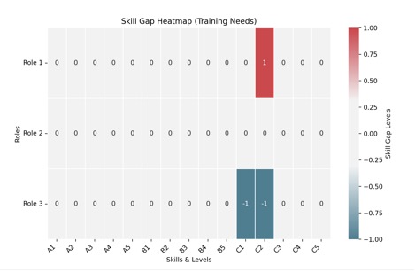
How to Interpret the Heatmap
- Rows: Different roles in the organization.
- Columns: Skill levels (1-5) for A, B, and C.
- Color Coding:
- Red (Positive Values): Training needed (skill is missing).
- White (Zero Values): Skill level is met.
- Blue (Negative Values): Overqualification (team exceeds the role’s needs).
This helps visualize where the largest training gaps exist so the team can focus on upskilling in specific skill levels.
Quantitative Risk Model
Risk Index = V(D) / V(R)
- Risk Index < 1: Highly controlled project
- Risk Index = 1: Balanced skill coverage
- Risk Index > 1: High potential for unmanaged complexity
Example Risk Scenarios
- V(D) = 3, V(R) = 3 → Risk Index = 1 (Balanced)
- V(D) = 6, V(R) = 3 → Risk Index = 2 (High Risk)
- V(D) = 9, V(R) = 3 → Risk Index = 3 (Critical Risk)
Same logic could be applied for H(V(D)) - H(V(R))
Works Cited
1. W Ross Ashby. An Introduction to Cybernetics. Chapman & Hall Ltd, 1961.
2. Ashby, W. R. (2011). Variety, Constraint, And The Law Of Requisite Variety. 13, 18.
3. Siegenfeld, A.F.; Bar-Yam, Y. A Formal Definition of Scale-dependent Complexity and the Multi-scale Law of Requisite Variety. arXiv 2022, arXiv:2206.04896.
Authors

Stoyan Boev

Dimitar Bakardzhiev
Getting started


